A short listing of resources useful for creating malware training sets for machine learning.

In leading academic and industry research on malware detection, it is common to use variations of the following techniques (based on Virustotal determinations) in order to build labeled training data.

–Jason
@jason_trost

The “short links” format was inspired by O’Reilly’s Four Short Links series.

In this post, I share my experience in building and maintaining large collections of benign IOCs (whitelists) for Threat Intelligence and Machine Learning Research.

Whitelisting is a useful concept in Threat Intelligence correlation since it can be very easy for benign observables to make their way into threat intelligence indicator feeds, esp. coming from open source providers or vendors that are not as careful as they should be. If these threat intelligence feeds are used for blocking (e.g. in firewalls or WAF devices) or alerting (e.g. log correlation in SIEM or IDS), the cost of benign entries making their way into a security control will be very high (wasted analyst time for triaging false positive alerts or loss of business productivity for blocked legitimate websites). Whitelists are generally used to filter out observables from threat intelligence feeds that almost certainly would be marked as a false positive if they were intersected against event logs (e.g. bluecoat proxy logs, firewall logs, etc) and used for alerting. Whitelists are also very useful for building labeled datasets required for building machine learning models and enriching alerts with contextual information.

The classic example of a benign observable is 8.8.8.8 (Google’s published open DNS resolver). This has found its way into many open source and commercial threat intelligence feeds by mistake since sometimes malware use this IP for DNS resolution or they ping it for connectivity checks. There are many other observables that commonly make their way into threat feeds due to how the threat feeds are derived / collected. Below are a summary of the major sources of false positives for threat intelligence feeds and ways to identify these to prevent their use. Most commercial threat intelligence platforms are pretty good at identifying these today and the dominant open source threat intelligence platform MISP is getting better with its MISP-warninglists, but as you will discover below there is some room for improvement.

Benign Inbound Observables

Benign Inbound Observables commonly show up in threat intelligence feeds derived from distributed network sensors such as honeypots or firewall logs. These IPs show up in firewall logs and are generally benign or at best are considered noise. Below are several common Benign Inbound Observable types. Each type also comes with recommended data sources or collection techniques listed as sub bullets:

  • Known Web Crawlers - Web crawlers are servers that crawl the World Wide Web and through this process may enter the networks of many companies or may accidentally hit honeypots or firewalls.
    • RDNS + DNS analytics can be used to enumerate these in bulk once patterns are identified. Here is an example pattern for googlebots. Mining large collections of rdns data can reveal other patterns to focus on. Below is an example of a simple PTR lookup on a known googlebot IP. This should start to reveal patterns that could be codified assuming you have access to a large corpus of RDNS data like is provided here (or could easily be generated).

Googlebot DNS

  • Known port scanners associated with highly visible projects or security companies (Shodan, Censys, Rapid7 Project Sonar, ShadowServer, etc.)
    • RDNS + DNS analytics may be able to enumerate these in bulk (assuming the vendors want to be identified). Example:

Shodan DNS

  • Mail Servers - these servers send email and they sometimes wind up on Threat feeds by mistake.
    • In order to enumerate these, you need a good list of popular email domains. Then perform DNS TXT request against this list and parse the SPF records. Multiple lookups will likely be needed as SPF allows for redirects and includes. Below shows the commands needed to do this manually for gmail.com as an example. The CIDR blocks returned are the IP space where gmail emails are sent from. Alerting or blocking on these is gonna cause a bad day.

Gmail DNS

  • Cloud PaaS Providers – Most Cloud providers publish their IP space via APIs or in their documentation. These lists are useful to derive whitelists, but they will need to be further filtered. Ideally you only whitelist Cloud IP space that are massively shared (like S3, CLOUDFRONT, etc), not IPs that are easy for bad guys to use, such as like EC2s. These whitelists should not be used to exclude domain names that resolve to this IP space, but instead should be used for either enrichments on alerting or to suppress IOC based alerting from these IP ranges.

Note: Greynoise is commercial provider of “anti-threat” intelligence (i.e. they identify the noise and other benign observables). They are very good at identifying the types of benign observables listed above since they maintain a globally distributed sensor array and are specifically analyzing network events in order to identify benign activity.

Note: MISP-warninglists provides many of these items today but they may be stale (several of their lists have not been updated in months). Ideally all of these lists are kept up-to-date through automated collection from authoritative sources instead of hard coded data stored in github (unless these are automatically updated frequently). See section on “Building / Maintaining Whitelist Data” for more tips.

Benign Outbound Observables

Benign Outbound Observables show up frequently in threat intelligence feeds derived from malware sandboxing, URL sandboxing, outbound web crawling, email sandboxing, and other similar threat feeds. Below are several common Benign Outbound Observable types. Each type also comes with recommended data sources or collection techniques listed as sub bullets:

  • Popular Domains - Popular domains can wind up on threat intelligence feeds, especially those derived from malware sandboxing since often times malware uses benign domains as connectivity checks and some malware, like those conducting click fraud act more like web crawlers, visiting many different benign sites. These same popular domains show up very often in most corporate networks and are almost always benign in nature (Note: they can be compromised and used for hosting malicious content so great care needs to be taken here).
  • Popular IP Addresses - Popular IPs are very similar to popular domains. They show up everywhere and when they wind up on threat intelligence feeds they cause a lot of false positives. Popular IP lists can be generated from resolving the Popular domain lists. These lists should not be used as-is for whitelisting; they need to be filtered/refined. See section on “Building / Maintaining Whitelist Data” below for more details on recommendations for refinement.
  • Free email domains - free email domains occasionally show up in threat intelligence feeds by accident so it is good to maintain a good list of these to prevent false positives. Hubspot provides a list that is decent.
  • Ad servers - Ad servers show up very frequently in URL sandbox feeds as these feeds are often obtained by visiting many websites and waiting for exploitation attempts or for AV alerts. These same servers show up all the time in benign Internet traffic. Easylist provides this sort of data.
  • CDN IPs - Content Distribution Networks are geographically distributed network of proxy servers or caches that provide high availability and high performance for web content distribution. Their servers are massively shared for distributing varied web content. When IPs from CDNs make it into threat intelligence feeds, false positives are soon to follow. Below are several CDN IP and domain sources.
  • Certificate Revocation Lists (CRL) and the Online Certificate Status Protocol (OCSP) domains/URLs - When executing a binary in a malware sandbox and the executable has been signed, connections will be made to CRL and OCSP servers. Because of this, these often mistakenly wind up in threat feeds.
    • Grab Certificates from Alexa top websites, extract OCSP URL. This old Alienvault post describes the process (along with another approach using the now defunct EFF SSL Observatory), and this github repo provides the code to do it. Care should be taken here since adversaries can influence the data collected in this way.
    • MISP-warninglists’ crl-ip-hostname
  • NTP Servers - Some malware call out to NTP servers for connectivity checks or to determine the real date/time. Because of this, NTP servers often wind up mistakenly on threat intelligence feeds that are derived from malware sandboxing.
  • Root Nameservers and TLD Nameservers
    • Perform DNS NS-lookups against each domain in the Public Suffix List and then perform DNS A-lookup each nameserver domain to obtain their IP addresses.
  • Mail Exchange servers
    • Obtain a list of popular email domains and then perform MX lookups against popular email domains to get their respective Mail Exchange (MX) servers. Perform DNS A-lookups on the MX servers list to obtain their IP addresses.
  • STUN Servers - “Session Traversal Utilities for NAT (STUN) is a standardized set of methods, including a network protocol, for traversal of network address translator (NAT) gateways in applications of real-time voice, video, messaging, and other interactive communications.” via https://en.wikipedia.org/wiki/STUN. Below are some sources of STUN servers (some of these appear old though).
  • Parking IPs - IPs used as the default IP for DNS-A records for brand new registered domains.
  • Popular Open DNS Resolvers
  • Security Companies, Security Blogs and Security Tool sites - These sites show up in threat mailing lists frequently which are sometimes scraped as threat feeds and these domains are mistakenly flagged as malicious.
  • Bit Torrent Trackers - github.com/ngosang/trackerslist
  • Tracking domains - commonly used by well known email marketing companies. Often shows up in threat intel feeds derived from spam or phishing email sinkholes. Results in high false positive rates in practice.
    • PDNS and/or Domain Whois analytics are one way to identify these once patterns can be observed. Below is an example of using Whois data for Marketo.com and identifying all the other Marketo email tracking domains that use Marketo’s nameserver. This example is from Whoisology, but bulk Whois mining is a preferred method.

Marketo Example

Note: MISP-warninglists provides some of these items today but they may be stale. Ideally all of these lists are kept up-to-date through automated collection from authoritative sources. See section on “Building / Maintaining Whitelist Data” for more tips.

Benign Host-based Observables

Benign Host-based Observables show up very commonly in threat intelligence feeds based on malware sandboxing. Here are some example observable types. So far, I have only found decent benign lists for File hashes (see below).

  • File hashes
  • Mutexes
  • Registry Keys
  • File Paths
  • Service names

Data Sources:

In leading academic and industry research on malware detection, it is common to use Virustotal in order to build labeled training data. See this post for more details. These techniques seem very suitable for training data creation, but are not recommended for whitelisting for operational use due to the high likelihood of false negatives.

Note: If your goal is building a machine learning model on binaries, you should strongly consider Endgame’s Ember. “The dataset includes features extracted from 1.1M binary files: 900K training samples (300K malicious, 300K benign, 300K unlabeled) and 200K test samples (100K malicious, 100K benign)”. See EMBER: An Open Dataset for Training Static PE Malware Machine Learning Models for more details.

Whitelist Exclusions

There are many observables that we will never want to whitelist due to their popularity or importance. These should be maintained in a whitelist exclusions list (a.k.a. greylist). Below are some examples:

Building / Maintaining Whitelist Data

Whitelist generation needs to be automated in order to be maintainable. There may be exceptions to this rule for things that you want to ensure are always in the whitelist, but for everything else, ideally they are collected from authoritative sources or are generated based on sound analytic techniques. You cannot always blindly trust each data source listed above. For several, some automated verification, filtering, or analytics will be needed. Below are some tips for how to do this effectively.

  • Each entity in the whitelist should be categorized (what type of whitelist entry is this?) and sourced (where did this come from?) so we know exactly how it got there (i.e. what data source was responsible) and when it was added/updated. This will help if there is ever a problem related to the whitelist so the specific source of the problem can be addressed.
  • Retrieve whitelist entries from the original source sites and parse/extract data from there. Avoid one time dumps of whitelist entries where possible since these will become stale very quickly. If you are including one-time dumps be sure to maintain their lineage.
  • Several bulk data sets will be very useful for analytics to expand or filter various whitelists
  • Netblock ownership (Maxmind) lookups / analytics will be useful for some of the vetting.
  • The whitelist should be updated at least daily to stay fresh. There may be data sources that change more or less frequently than this.
    • BE CAREFUL when refreshing the whitelist. Add sanity checks to ensure that the new whitelist was generated correctly before replacing the old one. The costs of a failed whitelist load will be mass false positives (unfortunately, I had to learn this lesson the hard way …).
  • Popular domain lists cannot be taken at face value as benign. Malicious domains get into these lists all the time. Here are some ways to combat this:
    • Use the N-day stable top-X technique - e.g. Stable 6-month Alexa top 500k - create a derivative list from the top Alexa domains where you filter the list for only domains that have been on the Alexa top 500k list every day for the past 6 months. This technique is commonly used in malicious domain detection literature as a way to build high quality benign labeled data. It is not perfect and may need to be tuned based on how the whitelist is being used. This technique requires keeping historic popular domain lists. The Wayback Machine appears to have a large historic mirror of the Alexa top1m data that may be suitable for bootstrapping your own collection.
  • Bulk DNS resolution of these lists can also be useful for generating Popular IP lists, but only when using the N-day stable top-X concept or if great care is taken in how they are used.
  • Use a whitelist exclusions set for removing categories of domains/IPs that you never want whitelisted. The whitelist exclusions set should also be kept fresh through automated collection from authoritative sources (e.g. scraping dynamic DNS providers and shared hosting websites where possible, PDNS / Whois analytics may also work).
  • Lastly, be careful when generating whitelists and think about what aspects of the data are adversary controlled. These are things we need to be careful not to blindly trust. Some examples:
    • RDNS entries can be made to be deceptive especially if the adversary knows they are used for whitelisting. For example, an adversary can create PTR records for IP address space they own that are identical to Google’s googlebot RDNS or Shodan’s census RDNS, BUT they cannot change the DNS A record mapping that domain name back to their IP space. For these a forward lookup (A Lookup) is generally also needed OR a netblock ownership verification.

In conclusion, whitelists are useful for filtering out observables from threat intelligence lists before correlation with event data, building labeled datasets for machine learning models, and enriching threat intelligence or alerts with contextual information. Creating and maintaining these lists can be a lot of work. Great care should be taken as to not go too far or to whitelist domains or IPs that are easily adversary controlled.

As always, feedback is welcome so please leave a message here, on Medium, or @ me on twitter!

–Jason
@jason_trost

This post explores Heterogeneous Information Networks (HIN) and applications to Cyber security.

Over the past few months I have been researching Heterogeneous Information Networks (HIN) and Cyber security use cases. I first encountered HIN’s after discovering this paper: “Gotcha: Sly Malware!- Scorpion A Metagraph2vec Based Malware Detection System” through a Google Scholar Alert I had setup for “Guilt by Association: Large Scale Malware Detection by Mining File-relation Graphs”. If you’re interested in how I setup my Google Alerts to stay abreast of the latest security data science research, see this: Security Data Science Learning Resources.

Heterogeneous Information Networks are a relatively simple way of modelling one or more datasets as a graph consisting of nodes and edges where 1) all nodes and edges have defined types, and 2) types of nodes > 1 or types of edges > 1 (hence “Heterogeneous”). The set of node and edge types represents the schema of the network. This differs from homogeneous networks where the nodes and edges are all the same type (e.g. Facebook Social Network Graph, World Wide Web, etc.). HINs provide a very rich abstraction for modelling complex datasets.

Below, I will walk through important HIN concepts using the HinDom paper as an example. HinDom uses DNS relationship data from passive DNS, DNS query logs, and DNS response logs to build a malicious domain classifier using HIN. They use Alexa Top 1K list, Malwaredomains.com, Malwaredomainlist.com, DGArchive, Google Safe Browsing, and VirusTotal for deriving labels. Below is an example HIN schema taken from this paper.

HinDom Schema

This schema represents three combined datasets (Passive DNS, DNS query logs, DNS response logs) and it models three node types (Client, Domain, and IP Address) and six edge types (segment, query, CNAME, similar, resolve, and same-domain). Here is an expanded example and descriptions of the relationships:

HinDom Example

  • Client-query-Domain - matrix Q denotes that domain i is queried by client j.
  • Client-segment-Client - matrix N denotes that client i and client j belong to the same network segment.
  • Domain-resolve-IP - matrix R denotes that domain i is resolved to IP address j.
  • Domain-similar-Domain - matrix S denotes the character-level similarity between domain i and j.
  • Domain-cname-Domain - matrix C denotes that domain i and domain j are in a CNAME record.
  • IP-domain-IP - matrix D denotes that IP address i and IP address j are once mapped to the same domain.

Once the dataset is represented as a graph, feature vectors need to be extracted before machine learning models can be built. A common technique for featurizing a HIN is by defining Meta-paths or Meta-graphs against the graph and then performing guided random walks against the defined meta-paths/graphs. Meta-paths represent graph traversals through specific node and edge sequences. Meta-paths selection are akin to feature engineering in classical machine learning as it is very important to select meta-paths that provide useful signals for whatever variable is being predicted. As seen in many HIN papers, meta-paths/graphs are often evaluated individually or in combination to determine their influence on model performance. Guided random walks against meta-paths produce a sequence of nodes (similar to sentences of words), which can then be fed into models like Skipgram or Continuous Bag-of-Words (CBOW) to create embeddings. Once the nodes are represented as embeddings many different models (SVM, DNN, etc) can be used to solve many different types of problems (Similarity Search, Classification, Clustering, Recommendation, etc). Below are the meta-paths used in the HinDom paper.

HinDom Meta-paths

Below is the HinDom Architecture to illustrate how all these concepts come together.

HinDom Architecture

Below are some resources that I found useful for learning more about Heterogeneous Information Networks as well as several security related papers that used HIN.

Books:

HIN Papers:

Malware Detection / Code Analysis:

Mining the Darkweb / Fraud Detection / Social Network Analysis:

Tutorials:

Code:

Prominent Security Researchers using HIN:


As always, feedback is welcome so please leave a message here, on Medium, or @ me on twitter!

–Jason
@jason_trost

This post outlines some experiments I ran using Auxiliary Loss Optimization for Hypothesis Augmentation (ALOHA) for DGA domain detection.

(Update 2019-07-18) After getting feedback from one of the ALOHA paper authors, I modified my code to set loss weights for the auxilary targets as they did in their paper (Weights used: main target 1.0, auxilary targets 0.1). I also added 3 word-based/dictionary DGAs. All diagrams and metrics have been updated to reflect this.

I recently read this paper ALOHA: Auxiliary Loss Optimization for Hypothesis Augmentation by Ethan M. Rudd, Felipe N. Ducau, Cody Wild, Konstantin Berlin, and Richard Harang from Sophos Lab. This research will be presented at USENIX Security 2019 in Aug, 2019. This paper shares findings that supplying more prediction targets to their model at training time, they can improve the prediction performance of the primary prediction target. More specifically, they modify a deep learning based model for detecting malware (binary classifier) to also predict things like individual vendor predictions, malware tags, and number of VT detections. Their “auxiliary loss architecture yields a significant reduction in detection error rate (false negatives) of 42.6% at a false positive rate (FPR) of 10^−3 when compared to a similar model with only one target, and a decrease of 53.8% at 10^−5 FPR.”

Aloha Model Architecture

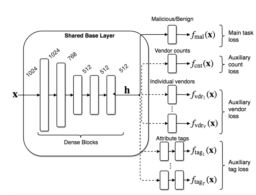
Figure 1 from the paper

A schematic overview of our neural network architecture. Multiple output layers with corresponding loss functions are optionally connected to a common base topology which consists of five dense blocks. Each block is composed of a Dropout, dense and batch normalization layers followed by an exponential linear unit (ELU) activation of sizes 1024, 768, 512, 512, and 512. This base, connected to our main malicious/benign output (solid line in the figure) with a loss on the aggregate label constitutes our baseline architecture. Auxiliary outputs and their respective losses are represented in dashed lines. The auxiliary losses fall into three types: count loss, multi-label vendor loss, and multi-label attribute tag loss

This paper made me wonder how well this technique would work for other areas in network security such as:

  • Detecting malicious URLs from Exploit Kits - possible auxiliary labels: Exploit Kit names, Web Proxy Categories, etc.
  • Detecting malicious C2 domains - possible auxiliary labels: malware family names, DGA or not, proxy categories.
  • Detecting DGA Domains - possible auxiliary labels: malware families, DGA type (wordlist, hex based, alphanumeric, etc).

I decided to explore the last use case of how well auxiliary loss optimizations would improve DGA domain detections. For this work I identified four DGA models and used these as baselines. Then I ran some experiments. All code from these experiments is hosted here. This code is based heavily off of Endgame’s dga_predict, but with many modifications.

Data:

For this work, I used the same data sources selected by Endgame’s dga_predict (but I added 3 additional DGAs: gozi, matsnu, and suppobox).

  • Alexa top 1m domains
  • classical DGA domains for the following malware families: banjori, corebot, cryptolocker, dircrypt, kraken, lockyv2, pykspa, qakbot, ramdo, ramnit, and simda.
  • Word-based/dictionary DGA domains for the following malware families - gozi, matsnu, and suppobox

Baseline Models:

I used 4 baseline binary models + 4 extensions of these model that use Auxiliary Loss Optimization for Hypothesis Augmentation.

Baseline Models:

ALOHA Extended Models (each simply use the 11 malware families as additional binary labels):

  • ALOHA CNN
  • ALOHA Bigram
  • ALOHA LSTM
  • ALOHA CNN+LSTM

I trained each of these models using the default settings as provided by dga_predict (except, I added stratified sampling based on the full labels: benign + malware families):

  • training splits: 76% training, 4% validation, %20 testing
  • all models were trained with a batch size of 128
  • The CNN, LSTM, and CNN+LSTM models used up to 25 epochs, while the bigram models used up to 50 epochs.

Below shows counts of how many of each DGA family were used and how many Alexa top 1m domains were included (denoted as “benign”).

1
2
3
4
5
6
7
8
9
10
11
12
13
14
15
16
17
18
19
20
21
22
23
24
In [1]: import pickle

In [2]: from collections import Counter

In [3]: data = pickle.loads(open('traindata.pkl', 'rb').read())

In [4]: Counter([d[0] for d in data]).most_common(100)
Out[4]: 
[('benign', 139935),
 ('qakbot', 10000),
 ('dircrypt', 10000),
 ('pykspa', 10000),
 ('corebot', 10000),
 ('kraken', 10000),
 ('suppobox', 10000),
 ('gozi', 10000),
 ('ramnit', 10000),
 ('matsnu', 10000),
 ('locky', 9999),
 ('banjori', 9984),
 ('simda', 9984),
 ('ramdo', 9984),
 ('cryptolocker', 9984)]

Results

Model AUC scores (sorted by AUC):

  • aloha_bigram 0.9435
  • bigram 0.9444
  • cnn 0.9817
  • aloha_cnn 0.9820
  • lstm 0.9944
  • aloha_cnn_lstm 0.9947
  • aloha_lstm 0.9950
  • cnn_lstm 0.9957

Overall, by AUC, the ALOHA technique only seemed to improve the LSTM and CNN models and only marginally. The ROC curves show reductions in the error rates at very low false positive rates (between 10^-5 and 10^-3) which is similar to those gains seen in the ALOHA paper, yet the paper’s gains appeared much larger.


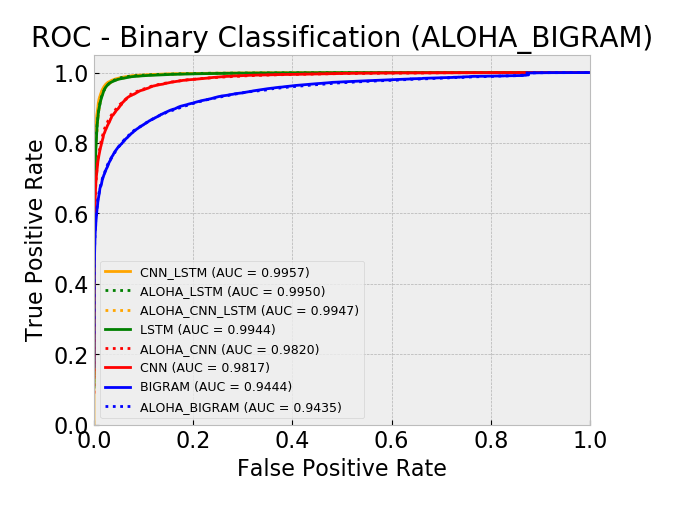
ROC: All Models Linear Scale


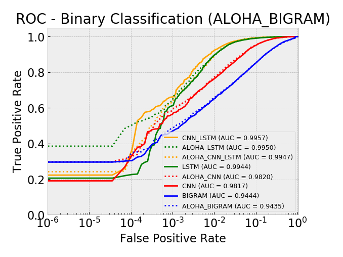
ROC: All Models Log Scale


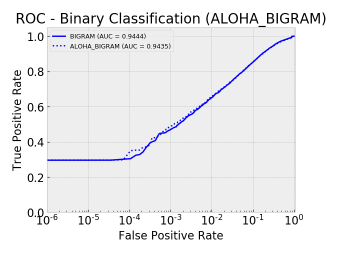
ROC: Bigram Models Log Scale


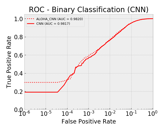
ROC: CNN Models Log Scale


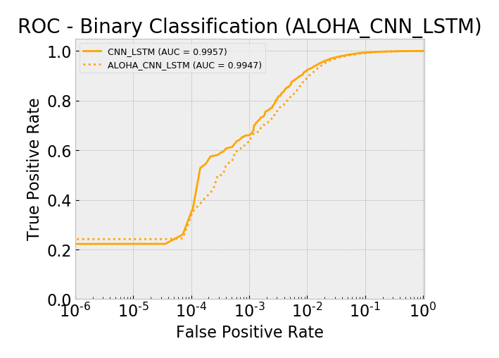
ROC: CNN+LSTM Models Log Scale


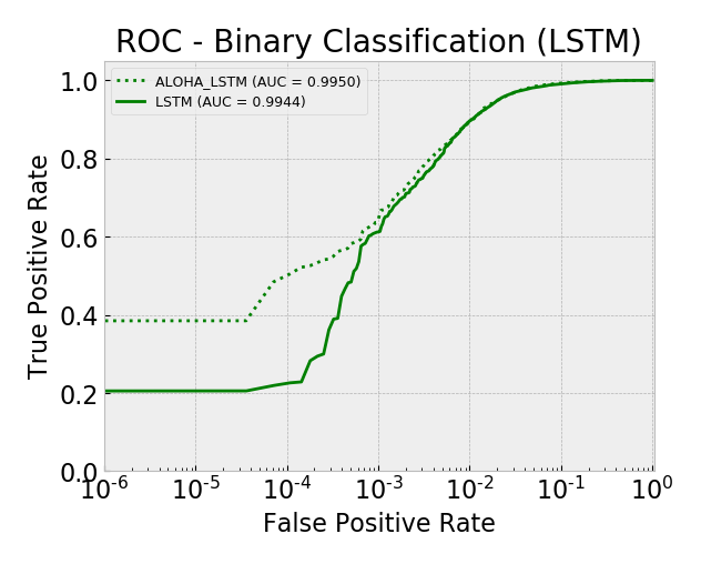
ROC: LSTM Models Log Scale
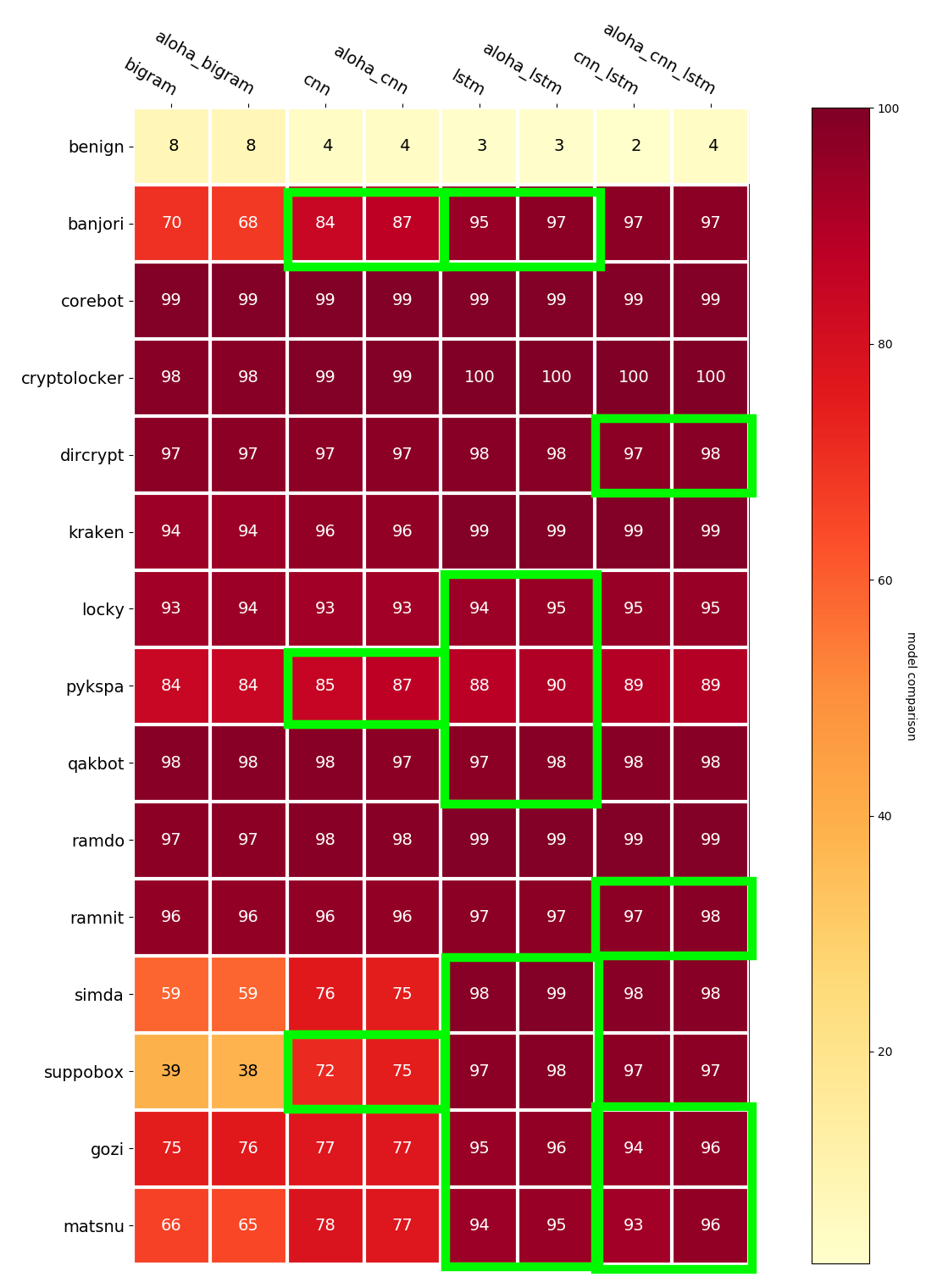
Heatmap

Below is a heatmap showing the percentage of detections across all the malware families for each model. Low numbers are good for the benign label (top row), high numbers are good for all the others.

Note the last 3 rows are all word-based/dictionary DGAs. It is interesting, although not too surprising that the models that include LSTMs tended to do better against these DGAs.

I annotated with green boxes places where the ALOHA models did better. This seems to be most apparent with the models that include LSTMs and for the word-based/dictionary DGAs.


Future Work:

These are some areas of future work I hope to have time to try out.

  • Add more DGA generators to the project, esp word-based / dictionary DGAs and see how the models react. I have identified several (see “Word-based / Dictionary-based DGA Resources” from here for more info).
  • try incorporating other auxiliary targets like:
    • Type of DGA (hex based, alphanumeric, custom alphabet, dictionary/word-based, etc)
    • Classical DGA domain features like string entropy, count of longest consecutive consonant string, count of longest consecutive vowel string, etc. I am curious if forcing the NN to learn these would improve its primary scoring mechanism.
    • Metadata from VT domain report.
    • Summary / stats from Passive DNS (PDNS).
    • Features from various aspects of the domain’s whois record.

If you enjoyed this post, you may be interested in my other recent post on Getting Started with DGA Domain Detection Research. Also, please see more Security Data Science blog posts at by personal blog: covert.io.

As always, feedback is welcome so please leave a message here, on Medium, or @ me on twitter!

–Jason
@jason_trost

This post provides resources for getting started with research on Domain Generation Algorithm (DGA) Domain Detection.

DGA Domains are commonly used by malware as a mechanism to maintain a command and control (C2) and make it more difficult for defenders to block. Prior to DGA domains, most malware used a small hardcoded list of IPs or domains. Once these IPs / domains were discovered they could be blocked by defenders or taken down for abuse. DGA domains make this more difficult since the C2 domain changes frequently and enumerating and blocking all generated domains can be expensive.

Recently, I have been working on a research project recently related to DGA detection (hopefully it will turn into a blogpost or a presentation somewhere), and it occurred to me that DGA is probably one of the most accessible areas for those getting into security data science due to the availability of so much labelled data and the availability of so many open source implementations of DGA detection. One might argue that this means it is not an area worth researching due to saturation, but I think that depends on your situation/goals. This short posts outlines some of the resources that I found useful for DGA research.

Data:

This section lists some domain lists and DGA generators that may be useful for creating “labelled” DGA domain lists.

DGA Data:

  • DGArchive Large private collection of DGA related data. This contains ~88 csv files of DGA domains organized by malware family. DGArchive is password protected and if you want access you need to reach out to the maintainer.
  • Bambenek Feeds (see “DGA Domain Feed”).
  • Netlab 360 DGA Feeds

DGA Generators:

Word-based / Dictionary-based DGA Resources:

Below are all Malware Families that use word-based / dictionary DGAs, meaning their domains consist of 2 or more words selected from a list/dictionary and concatenated together. I separate these out since they are different than most other “classical” DGAs.

“Benign” / Non-DGA Data:

This section lists some domain lists that may be useful for creating “labelled” benign domain lists. In several academic papers one or more of these sources are used, but they generally create derivatives that represent the Stable N-day Top X Sites (e.g. Stable Alexa 30-day top 500k – meaning domains from the Alexa top 500k that have been on the list consecutively for the last 30 days straight – the alexa data needs to be downloaded each day for 30+ days to create this since only today’s snapshot is provided by Amazon). This filters out domains that can become popular for a short amount of time but them drop off as sometimes happens with malicious domains.

Update (2020-03-22) - More Heuristics for Benign training set curation:

Excerpt from Inline Detection of DGA Domains Using Side Information (page 12)

The benign samples are collected based on a predefined set of heuristics as listed below:

  • Domain name should have valid DNS characters only (digits, letters, dot and hyphen)
  • Domain has to be resolved at least once for every day between June 01, 2019 and July 31, 2019.
  • Domain name should have a valid public suffix
  • Characters in the domain name are not all digits (after removing ‘.’ and ‘-‘)
  • Domain should have at most four labels (Labels are sequence of characters separated by a dot)
  • Length of the domain name is at most 255 characters
  • Longest label is between 7 and 64 characters
  • Longest label is more than twice the length of the TLD
  • Longest label is more than 70% of the combined length of all labels
  • Excludes IDN (International Distribution Network) domains (such as domains starting with xn–)
  • Domain must not exist in DGArchive

Utilities:

Domain Parser:

When parsing the various domain list data tldextract is very helpful for stripping off TLDs or subdomains if desired. I have seen several projects attempt to parse domains using “split(‘.’)” or “domain[:-3]”. This does not work very well since domain’s TLDs can contain multiple “.”s (e.g. .co.uk)

Installation:

1
pip install tldextract

Example:

1
2
3
4
5
6
7
8
9
10
11
12
13
14
15
16
17
18
19
In [1]: import tldextract
In [2]: e = tldextract.extract('abc.www.google.co.uk')

In [3]: e                                                                                                                            Out[3]: ExtractResult(subdomain='abc.www', domain='google', suffix='co.uk')

In [4]: e.domain
Out[4]: 'google'

In [5]: e.subdomain
Out[5]: 'abc.www'

In [6]: e.registered_domain
Out[6]: 'google.co.uk'

In [7]: e.fqdn
Out[7]: 'abc.www.google.co.uk'

In [8]: e.suffix
Out[8]: 'co.uk'

Domain Resolution:

During the course of your research you may need to perform DNS resolutions on lots of DGA domains. If you do this, I highly recommend setting up your own bind9 server on Digital Ocean or Amazon and using adnshost (a utility from adns). If you perform the DNS resolutions from your home or office, your ISP may interfere with the DNS responses because they will appear malicious, which can bias your research. If you use a provider’s recursive nameservers, you may violate the acceptable use policy (AUP) due to the volume AND the provider may also interfere with the responses.

Adnshost enables high throughput / bulk DNS queries to be performed asynchronously. It will be much faster than performing the DNS queries synchronously (one after the other).

Here is an example of using adnshost (assuming you are running it from the Bind9 server you setup):

1
2
3
4
5
6
cat huge-domains-list.txt | adnshost \
    --asynch \
    --config "nameserver 127.0.0.1" \
    --type a \
    --pipe \
    ----addr-ipv4-only > results.txt

This article should get you most of the way there with setting up the bind9 server.

Models:

This section provides links to a few models that could be used as baselines for comparison.

Research:


I hope this is helpful. As always, feedback is welcome so please leave a message here, on Medium, or @ me on twitter!

–Jason
@jason_trost